How to set plot colors in Matplotlib

Color choices in a Matplotlib figure separate related data series, keep markers readable, and make a chart match a report palette. Assigning explicit color values to the artists keeps the chosen palette unchanged when a style sheet or project-level property cycle supplies different defaults.

Color specifications in Matplotlib include named colors, hexadecimal strings, RGB or RGBA tuples with values from 0 to 1, grayscale strings, and property-cycle references. Named colors, hex values, and tuples resolve directly, while references such as C2 look up the active property cycle and therefore do not belong in a fixed palette.

Direct artist colors suit fixed categories or brand colors. Use a colormap instead when numeric values should select colors from a scale, or a style sheet when the same defaults should apply across many figures.

1. Define the sample series, non-default style, and fixed palette in plot_color_set.py.

   plot_color_set.py

   import matplotlib.pyplot as plt
   from matplotlib.colors import to_hex
    
   plt.style.use("ggplot")
    
   months = ["Jan", "Feb", "Mar", "Apr", "May"]
   planned = [4, 5, 6, 7, 8]
   actual = [3, 6, 5, 8, 9]
    
   palette = {
       "line": "tab:blue",
       "marker_face": "#ffbf00",
       "marker_edge": (0.0, 0.2, 0.4),
       "bars": "#2ca02c",
       "fill": (0.2, 0.6, 0.9, 0.25),
   }

   The non-default ggplot style changes the chart defaults, while the palette uses a Tableau color name, explicit hex values, an RGB tuple, and an RGBA tuple with transparency.

2. Append the figure and colored line artist to plot_color_set.py.

   fig, ax = plt.subplots(layout="constrained")
    
   (actual_line,) = ax.plot(
       months,
       actual,
       color=palette["line"],
       marker="o",
       markerfacecolor=palette["marker_face"],
       markeredgecolor=palette["marker_edge"],
       linewidth=2.5,
       label="Actual",
   )

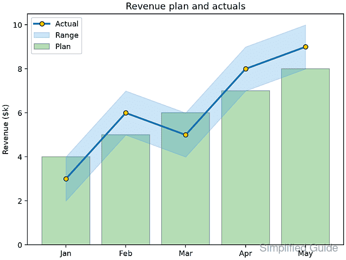
   color controls the line, while markerfacecolor and markeredgecolor set the marker fill and outline independently.

3. Append the colored bars and translucent range to plot_color_set.py.

   bars = ax.bar(
       months,
       planned,
       color=palette["bars"],
       edgecolor="#1f2937",
       alpha=0.35,
       label="Plan",
   )
    
   band = ax.fill_between(
       months,
       [value - 1 for value in actual],
       [value + 1 for value in actual],
       color=palette["fill"],
       label="Range",
   )

   The explicit #2ca02c value keeps the bar faces green instead of taking a color from the active style. The four-value fill tuple carries its own alpha channel for the range.

4. Append the chart labels and legend to plot_color_set.py.

   ax.set_title("Revenue plan and actuals")
   ax.set_ylabel("Revenue ($k)")
   ax.legend()

5. Append the PNG export and resolved-color report to plot_color_set.py.

   fig.savefig("plot-color-set.png", dpi=160)
    
   print(f"line color: {to_hex(actual_line.get_color())}")
   print(f"marker face: {to_hex(actual_line.get_markerfacecolor())}")
   print(f"marker edge: {to_hex(actual_line.get_markeredgecolor())}")
   print(f"bar face: {to_hex(bars.patches[0].get_facecolor())}")
   print(f"fill face: {to_hex(band.get_facecolor()[0], keep_alpha=True)}")
   print("saved: plot-color-set.png")
    
   plt.close(fig)

6. Run plot_color_set.py from the directory that should receive the PNG.

   $ python3 plot_color_set.py
   line color: #1f77b4
   marker face: #ffbf00
   marker edge: #003366
   bar face: #2ca02c
   fill face: #3399e640
   saved: plot-color-set.png

7. Confirm plot-color-set.png shows the blue line, amber markers, green bars, and translucent blue range under the active ggplot style.