Many time-dependent systems begin with a known state and a rule for its rate of change. SciPy represents that problem as a first-order state vector and advances it numerically across a specified time interval.
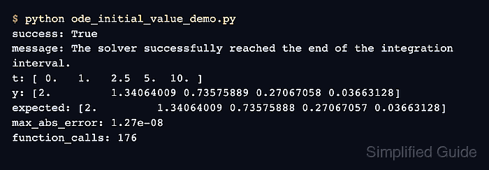
The scipy.integrate.solve_ivp() function expects a derivative callable with the signature fun(t, y), an integration interval, and an initial state. Its t_eval argument selects the times returned in solution.t and the matching state columns stored in solution.y.
An exponential decay model has the analytic solution y(t) = 2e^-0.4t, so it can expose an incorrect derivative, state index, or time span. A numerical assertion against that solution provides fail-capable proof in addition to the solver's own completion status.
Steps to solve a SciPy ODE initial value problem:
- Create ode_initial_value_demo.py with the decay model and initial state.
- ode_initial_value_demo.py
import numpy as np
from scipy.integrate import solve_ivp


DECAY_RATE = 0.4
INITIAL_VALUE = 2.0


def exponential_decay(t, y):
    return [-DECAY_RATE * y[0]]
The derivative returns one value because y0 will contain one state variable.
- Append the integration interval and requested sample times below the derivative function.
- ode_initial_value_demo.py
time_span = (0.0, 10.0)
sample_times = np.array([0.0, 1.0, 2.5, 5.0, 10.0])
t_eval controls the returned sample grid; the solver still chooses its internal integration steps.
- Append the solve_ivp() call below the sample-time array.
- ode_initial_value_demo.py
solution = solve_ivp(
    exponential_decay,
    t_span=time_span,
    y0=[INITIAL_VALUE],
    t_eval=sample_times,
    method="RK45",
    rtol=1e-8,
    atol=1e-10,
)
RK45 is intended for non-stiff equations such as this decay model. Radau or BDF may be more suitable when a model is stiff.
- Append fail-capable result checks and summary output below the solver call.
- ode_initial_value_demo.py
if not solution.success:
    raise RuntimeError(solution.message)

expected = INITIAL_VALUE * np.exp(-DECAY_RATE * sample_times)
np.testing.assert_allclose(solution.y[0], expected, rtol=1e-7, atol=1e-9)

if not np.isclose(solution.t[-1], time_span[1]):
    raise RuntimeError("The solver stopped before the final time.")

max_abs_error = np.max(np.abs(solution.y[0] - expected))
print(f"time: {np.array2string(solution.t, precision=2)}")
print(f"state: {np.array2string(solution.y[0], precision=8)}")
print(f"max_abs_error: {max_abs_error:.2e}")
print(f"final_time: {solution.t[-1]:.1f}")
print(f"solver_message: {solution.message}")
solution.y[0] selects the first state variable across every requested time. Either assertion stops the program before it can print a successful result when the integration is wrong.
- Run the completed initial value program.
$ python ode_initial_value_demo.py
time: [ 0.   1.   2.5  5.  10. ]
state: [2.         1.34064009 0.73575888 0.27067057 0.03663128]
max_abs_error: 1.11e-09
final_time: 10.0
solver_message: The solver successfully reached the end of the integration interval.

Mohd Shakir Zakaria is a cloud architect with deep roots in software development and open-source advocacy. Certified in AWS, Red Hat, VMware, ITIL, and Linux, he specializes in designing and managing robust cloud and on-premises infrastructures.


