How to set a log axis scale in Matplotlib

Linear axes make equal numeric gaps look equal, which can bury patterns when a Matplotlib plot spans several powers of ten. A logarithmic axis spaces ticks by ratio, so growth from 100 to 1,000 uses the same visual interval as growth from 10,000 to 100,000.

The object-oriented Axes API keeps the scale change attached to one subplot. Use ax.set_yscale(“log”) for vertical values or ax.set_xscale(“log”) for horizontal values; the example changes only the y-axis so the year labels remain linear.

Use positive values when every point must remain visible on a standard logarithmic axis. Matplotlib places major ticks at powers of 10 and clips non-positive values by default, while symlog adds a linear region around zero when the plot must retain values on both sides of zero.

1. Create log_axis_scale.py with the positive request values used by the logarithmic y-axis.

   log_axis_scale.py

   import matplotlib.pyplot as plt
    
   years = [2022, 2023, 2024, 2025, 2026]
   requests = [250, 1800, 12600, 94000, 710000]

   The default logarithmic transform clips values at zero or below; filter, mask, or use symlog when those values must remain visible.

2. Append the Axes construction and line plot below the request values.

   fig, ax = plt.subplots(layout="constrained")
   ax.plot(years, requests, marker="o")

3. Append the logarithmic y-axis setting immediately after the line plot.

   ax.set_yscale("log")

4. Append the plot presentation section below the scale setting.

   ax.set_xticks(years)
   ax.set_xlabel("Year")
   ax.set_ylabel("Requests")
   ax.set_title("Requests by year")
   ax.grid(True, which="both", axis="y", color="0.9")

5. Append the scale check and PNG export below the grid setting.

   x_scale = ax.get_xscale()
   y_scale = ax.get_yscale()
    
   assert x_scale == "linear"
   assert y_scale == "log"
    
   fig.savefig("requests-log-axis.png", dpi=150)
    
   print(f"x scale: {x_scale}")
   print(f"y scale: {y_scale}")
   print("saved: requests-log-axis.png")

6. Compare the assembled log_axis_scale.py file with the complete script.

   log_axis_scale.py

   import matplotlib.pyplot as plt
    
   years = [2022, 2023, 2024, 2025, 2026]
   requests = [250, 1800, 12600, 94000, 710000]
    
   fig, ax = plt.subplots(layout="constrained")
   ax.plot(years, requests, marker="o")
    
   ax.set_yscale("log")
    
   ax.set_xticks(years)
   ax.set_xlabel("Year")
   ax.set_ylabel("Requests")
   ax.set_title("Requests by year")
   ax.grid(True, which="both", axis="y", color="0.9")
    
   x_scale = ax.get_xscale()
   y_scale = ax.get_yscale()
    
   assert x_scale == "linear"
   assert y_scale == "log"
    
   fig.savefig("requests-log-axis.png", dpi=150)
    
   print(f"x scale: {x_scale}")
   print(f"y scale: {y_scale}")
   print("saved: requests-log-axis.png")

7. Run log_axis_scale.py from the Python environment that has Matplotlib installed.

   $ python log_axis_scale.py
   x scale: linear
   y scale: log
   saved: requests-log-axis.png

8. Confirm the saved plot uses powers-of-ten tick spacing on the y-axis.

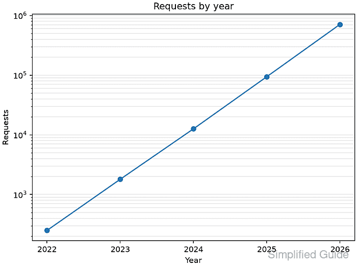
   The printed y scale: log value identifies the active scale, and equal vertical intervals in the saved plot represent equal ratios.