How to explain a Spark DataFrame query plan

Spark builds a query plan before a DataFrame action distributes work across executors. Reading that plan exposes the filters, projections, aggregations, shuffles, and sorting Spark expects to perform, which helps distinguish an expensive transformation shape from a problem in the surrounding job.

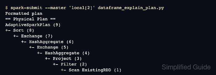
The DataFrame.explain() method can show the plan at different levels. formatted mode pairs a compact physical operator tree with details for each numbered node, while extended mode shows how the parsed expression becomes an analyzed plan, an optimized logical plan, and executable physical operators.

Generated attribute numbers, plan IDs, and adaptive-plan details can differ across Spark releases or session settings. Match operator names to the transformation first, then use Exchange boundaries, aggregate stages, projections, and pushed filters to understand where Spark will move or reduce data.

1. Create dataframe_explain_plan.py with the Spark session configuration.

   dataframe_explain_plan.py

   from pyspark.sql import SparkSession
   from pyspark.sql import functions as F
    
    
   spark = (
       SparkSession.builder.appName("dataframe-explain-plan")
       .config("spark.ui.enabled", "false")
       .config("spark.sql.adaptive.enabled", "true")
       .getOrCreate()
   )
   spark.sparkContext.setLogLevel("ERROR")

2. Add the input rows that establish the region, team, and amount columns.

   dataframe_explain_plan.py

   orders = spark.createDataFrame(
       [
           ("EMEA", "analytics", 1200),
           ("EMEA", "analytics", 800),
           ("APAC", "platform", 500),
           ("EMEA", "platform", 700),
           ("AMER", "analytics", 400),
       ],
       ["region", "team", "amount"],
   )

   Related: How to create a Spark DataFrame

3. Define the totals DataFrame with the filter, grouped sum, and descending sort.

   dataframe_explain_plan.py

   totals = (
       orders.filter(F.col("region") == "EMEA")
       .groupBy("team")
       .agg(F.sum("amount").alias("total_amount"))
       .orderBy(F.col("total_amount").desc())
   )

   Related: How to select and filter a Spark DataFrame

4. Append the formatted physical-plan view below the transformation.

   dataframe_explain_plan.py

   print("Formatted plan")
   totals.explain(mode="formatted")

5. Append the extended logical-plan view below the formatted call.

   dataframe_explain_plan.py

   print("Extended plan")
   totals.explain(mode="extended")

   simple prints only the physical plan. cost adds logical-plan statistics when Spark has them, while codegen prints generated code for supported physical operators.

6. Add the result action below both plan views.

   dataframe_explain_plan.py

   print("Result rows")
   totals.show()

7. Finish the script with the Spark session shutdown.

   dataframe_explain_plan.py

   spark.stop()

8. Submit the completed script to a local Spark master.

   $ spark-submit --master 'local[2]' dataframe_explain_plan.py
   Formatted plan
   == Physical Plan ==
   AdaptiveSparkPlan (9)
   +- Sort (8)
      +- Exchange (7)
         +- HashAggregate (6)
            +- Exchange (5)
               +- HashAggregate (4)
                  +- Project (3)
                     +- Filter (2)
                        +- Scan ExistingRDD (1)
   
   ##### snipped #####

9. Trace the formatted physical plan upward from Scan ExistingRDD to Sort.

   In this plan, Filter represents the region == “EMEA” condition, while Project retains only columns needed later. The two HashAggregate nodes perform partial and final aggregation. Each Exchange marks a shuffle boundary, while Sort orders the aggregated rows.

10. Compare the parsed plan with the optimized logical plan in the extended output.

    Extended plan
    == Parsed Logical Plan ==
    'Sort ['total_amount DESC NULLS LAST], true
    +- Aggregate [team#1], [team#1, sum(amount#2L) AS total_amount#3L]
       +- Filter (region#0 = EMEA)
          +- LogicalRDD [region#0, team#1, amount#2L], false
    
    ##### snipped #####
    
    == Optimized Logical Plan ==
    Sort [total_amount#3L DESC NULLS LAST], true
    +- Aggregate [team#1], [team#1, sum(amount#2L) AS total_amount#3L]
       +- Project [team#1, amount#2L]
          +- Filter (isnotnull(region#0) AND (region#0 = EMEA))
             +- LogicalRDD [region#0, team#1, amount#2L], false
    
    ##### snipped #####

    The optimized plan adds a null check and prunes region before aggregation. The physical section chooses executable operators and inserts shuffle boundaries for the grouped sum and global ordering.
    Related: How to configure Spark adaptive query execution

11. Confirm that the action returns the rows represented by the inspected plan.

    Result rows
    +---------+------------+
    |     team|total_amount|
    +---------+------------+
    |analytics|        2000|
    | platform|         700|
    +---------+------------+