How to train logistic regression with scikit-learn
A classification model earns its place by predicting labels for examples it did not see during fitting. scikit-learn provides LogisticRegression as a compact linear baseline for labeled numeric data, with predicted labels and class probabilities available through the estimator API.
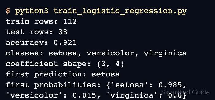
The Iris dataset supplies three species and four numeric flower measurements. A fixed stratified split reserves 25 percent of its rows for testing while preserving the species mix, so the fitted model is evaluated against data excluded from training.
Placing StandardScaler and LogisticRegression in the same Pipeline prevents the scaler from learning from the test partition. The completed model can then apply that fitted transformation consistently when it scores the held-out rows and predicts an unseen flower.
Steps to train a scikit-learn logistic regression model:
- Create train_logistic_regression.py with the imports and stratified Iris train/test split.
- train_logistic_regression.py
from sklearn.datasets import load_iris
from sklearn.linear_model import LogisticRegression
from sklearn.model_selection import train_test_split
from sklearn.pipeline import make_pipeline
from sklearn.preprocessing import StandardScaler


iris = load_iris()
X_train, X_test, y_train, y_test = train_test_split(
    iris.data,
    iris.target,
    test_size=0.25,
    stratify=iris.target,
    random_state=42,
)
- Append the scaled logistic regression pipeline after the train/test split.
model = make_pipeline(
    StandardScaler(),
    LogisticRegression(max_iter=200),
)
model.fit(X_train, y_train)
The pipeline fits StandardScaler from X_train and applies the learned transformation automatically during prediction.
Related: How to create a scikit-learn pipeline
Related: How to standardize features with scikit-learn - Append the held-out evaluation block beneath the existing pipeline section.
accuracy = model.score(X_test, y_test)
sample = X_test[[0]]
prediction = model.predict(sample)[0]
probabilities = model.predict_proba(sample)[0]

assert accuracy >= 0.90
assert abs(probabilities.sum() - 1.0) < 1e-12

class_probabilities = {
    str(name): round(float(probability), 3)
    for name, probability in zip(iris.target_names, probabilities)
}

print(f"training rows: {len(X_train)}")
print(f"test rows: {len(X_test)}")
print(f"held-out accuracy: {accuracy:.3f}")
print(f"predicted species: {iris.target_names[prediction]}")
print(f"class probabilities: {class_probabilities}")
print(f"probability sum: {probabilities.sum():.3f}")
The assertions make the run fail if held-out accuracy drops below 0.90 or the predicted class probabilities stop forming a complete distribution.
- Run the completed logistic regression script from the directory that contains it.
$ python3 train_logistic_regression.py
training rows: 112
test rows: 38
held-out accuracy: 0.921
predicted species: setosa
class probabilities: {'setosa': 0.985, 'versicolor': 0.015, 'virginica': 0.0}
probability sum: 1.000
The observed score comes from 38 held-out rows, while the prediction and probability output exercise the fitted pipeline on one unseen flower.