How to create a histogram in Matplotlib
Numeric measurements can hide their distribution behind a single average or total. A histogram exposes clusters, gaps, and skew by grouping observations into intervals and drawing the frequency of each interval.
The Matplotlib Axes.hist() method accepts the raw observations and a sequence of bin edges. Explicit edges make the interval boundaries predictable, including the final interval's right edge, and keep the same grouping when the script is rerun.
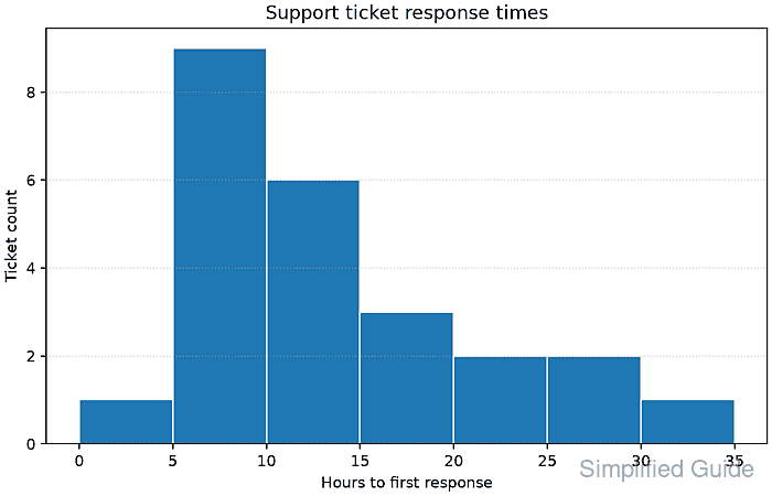
The completed plot reports how many observations reached each bin before saving the figure as a PNG. Matching the counted total to the input size catches values that fall outside the selected edge range, while the rendered bars reveal the distribution itself.
Related: How to create a box plot in Matplotlib
Related: How to create a bar chart in Matplotlib
Related: How to set axis labels in Matplotlib
Steps to create a Matplotlib histogram:
- Create create_histogram.py with the imports, observations, and explicit bin edges.
- create_histogram.py
from pathlib import Path

import matplotlib.pyplot as plt

response_hours = [
    4, 5, 5, 6, 7, 7, 8, 9,
    9, 9, 10, 11, 12, 12, 13, 14,
    15, 16, 18, 20, 22, 25, 28, 31,
]
bin_edges = [0, 5, 10, 15, 20, 25, 30, 35]
The supplied edges cover the full data range. Every interval except the last excludes its right edge, while the last interval includes both edges.
- Append the histogram calculation and bar styling to create_histogram.py.
fig, ax = plt.subplots(figsize=(7, 4.5), layout="constrained")
counts, edges, _ = ax.hist(
    response_hours,
    bins=bin_edges,
    color="tab:blue",
    edgecolor="white",
)
Axes.hist() returns the bin counts, bin edges, and the artists used to draw the bars.
- Append the final labeled-figure export section to create_histogram.py.
ax.set_title("Support ticket response times")
ax.set_xlabel("Hours to first response")
ax.set_ylabel("Ticket count")
ax.set_xticks(bin_edges)
ax.grid(axis="y", linestyle=":", alpha=0.5)

output = Path("ticket-response-histogram.png")
fig.savefig(output, dpi=160)
plt.close(fig)

print(f"samples: {len(response_hours)}")
print(f"bins: {len(edges) - 1}")
print(f"counts: {[int(count) for count in counts]}")
print(f"counted samples: {int(counts.sum())}")
print(f"saved: {output}")
print(f"bytes: {output.stat().st_size}")
- Run create_histogram.py from the Python environment that has Matplotlib installed.
$ python3 create_histogram.py
samples: 24
bins: 7
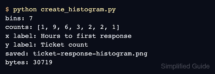
counts: [1, 9, 6, 3, 2, 2, 1]
counted samples: 24
saved: ticket-response-histogram.png
bytes: 30800
The byte count can differ with the Matplotlib version, fonts, backend, and DPI. The counted total should equal the number of input observations.
- Open ticket-response-histogram.png to confirm that the chart contains seven bars and peaks in the 5-to-10-hour interval.