How to train a demand forecast model in Keras
Short-term demand forecasts depend on time order: yesterday can inform tomorrow, but tomorrow must never leak into training. A compact Keras model can turn recent demand, promotion timing, and weekly seasonality into a saved forecasting artifact while preserving that boundary.
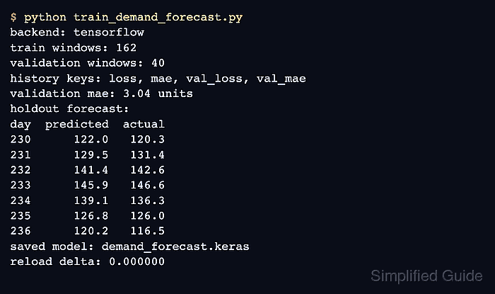
The sample builds one-step forecasts from 28-day windows. It calculates normalization values from the training period, reserves the next 40 target days for validation, and leaves the final 30 target days as an untouched holdout.
Synthetic demand keeps the first run reproducible without exposing business data. Replace those generated rows only after the chronological split works, and retain the same feature availability rule so every value in a window would have been known before its target day.
Steps to train a Keras demand forecast model:
- Install Keras, TensorFlow, and NumPy in the project environment.
$ python -m pip install keras tensorflow numpy
An isolated virtual environment keeps project dependencies separate. Standalone Keras reads KERAS_BACKEND before import keras.
Related: How to install Keras with pip - Create train_demand_forecast.py with the imports, chronological boundaries, and time-ordered feature rows.
- train_demand_forecast.py
import os

os.environ["KERAS_BACKEND"] = "tensorflow"
os.environ["TF_CPP_MIN_LOG_LEVEL"] = "2"

from pathlib import Path

import keras
import numpy as np
from keras import layers

LOOKBACK = 28
TRAIN_END = 190
VALIDATION_END = 230
MODEL_PATH = Path("demand_forecast.keras")

keras.utils.set_random_seed(7)

rng = np.random.default_rng(42)
days = np.arange(260, dtype="float32")
weekly = 12.0 * np.sin(2.0 * np.pi * days / 7.0)
trend = 0.08 * days
promotion = ((days % 31) < 4).astype("float32")
noise = rng.normal(0.0, 2.0, size=days.shape[0]).astype("float32")
demand = 120.0 + trend + weekly + (18.0 * promotion) + noise

train_mean = demand[:TRAIN_END].mean()
train_std = demand[:TRAIN_END].std()
demand_scaled = (demand - train_mean) / train_std

features = np.column_stack(
    [
        demand_scaled,
        promotion,
        np.sin(2.0 * np.pi * days / 7.0),
        np.cos(2.0 * np.pi * days / 7.0),
    ]
).astype("float32")
The synthetic series combines trend, weekly seasonality, promotions, and noise. Scaling uses only rows before TRAIN_END so later demand cannot influence training statistics.
- Append the window builder and chronological masks below the feature rows.
- train_demand_forecast.py
def make_windows(feature_rows, target_values, lookback):
    windows = []
    targets = []
    target_days = []
    for start in range(len(feature_rows) - lookback):
        target_day = start + lookback
        windows.append(feature_rows[start:target_day])
        targets.append(target_values[target_day])
        target_days.append(target_day)
    return (
        np.asarray(windows, dtype="float32"),
        np.asarray(targets, dtype="float32"),
        np.asarray(target_days, dtype="int32"),
    )


x_all, y_all, target_days = make_windows(features, demand_scaled, LOOKBACK)
train_mask = target_days < TRAIN_END
validation_mask = (target_days >= TRAIN_END) & (target_days < VALIDATION_END)
holdout_mask = target_days >= VALIDATION_END

x_train, y_train = x_all[train_mask], y_all[train_mask]
x_val, y_val = x_all[validation_mask], y_all[validation_mask]
x_holdout, y_holdout = x_all[holdout_mask], y_all[holdout_mask]
holdout_days = target_days[holdout_mask]
Each target follows its 28 input rows. The masks use target-day numbers rather than shuffled row counts, which keeps validation and holdout targets later than every training target.
- Append the LSTM model, training call, holdout forecast, and saved-model reload below the split.
- train_demand_forecast.py
model = keras.Sequential(
    [
        layers.Input(shape=(LOOKBACK, features.shape[1])),
        layers.LSTM(24),
        layers.Dense(12, activation="relu"),
        layers.Dense(1),
    ]
)
model.compile(
    optimizer=keras.optimizers.Adam(learning_rate=0.01),
    loss="mse",
    metrics=[keras.metrics.MeanAbsoluteError(name="mae")],
)

model.fit(
    x_train,
    y_train,
    validation_data=(x_val, y_val),
    epochs=8,
    batch_size=32,
    shuffle=False,
    verbose=0,
)

validation_metrics = model.evaluate(x_val, y_val, verbose=0, return_dict=True)
forecast_scaled = model.predict(x_holdout[:7], verbose=0).reshape(-1)
forecast = (forecast_scaled * train_std) + train_mean
actual = (y_holdout[:7] * train_std) + train_mean
holdout_mae = np.mean(np.abs(forecast - actual))

model.save(MODEL_PATH)
reloaded = keras.saving.load_model(MODEL_PATH)
reloaded_forecast = reloaded.predict(x_holdout[:1], verbose=0).reshape(-1)[0]
reload_delta = abs(reloaded_forecast - forecast_scaled[0])
assert reload_delta < 1e-6

print(f"backend: {keras.backend.backend()}")
print(f"train windows: {x_train.shape[0]}")
print(f"validation windows: {x_val.shape[0]}")
print(f"validation mae: {validation_metrics['mae'] * train_std:.2f} units")
print(f"holdout mae: {holdout_mae:.2f} units")
print("day  predicted  actual")
for day, predicted, observed in zip(holdout_days[:7], forecast, actual):
    print(f"{int(day):3d}  {predicted:9.1f}  {observed:6.1f}")
print(f"saved model: {MODEL_PATH}")
print(f"reload delta: {reload_delta:.6f}")
validation_data measures later rows during training, while the holdout remains unused until the final forecast. The .keras file stores model configuration, weights, and optimizer state.
Related: How to save and load a Keras model - Check the trained model against later demand with the completed training program.
$ python train_demand_forecast.py
backend: tensorflow
train windows: 162
validation windows: 40
validation mae: 3.65 units
holdout mae: 3.01 units
day  predicted  actual
230      131.1   126.1
231      141.3   137.3
232      148.7   148.6
233      150.0   152.8
234      145.6   142.5
235      133.7   132.3
236      127.5   122.9
saved model: demand_forecast.keras
reload delta: 0.000000
The validation and holdout errors are expressed in the original demand units. A zero reload delta confirms that the saved artifact reproduces the first holdout forecast; real data still needs a business-specific error threshold before deployment.