How to train a random forest with scikit-learn
Random forests combine predictions from many randomized decision trees, making them a useful baseline when tabular classification depends on nonlinear relationships or feature interactions. A fitted forest can predict without feature scaling, while its tree count and depth still need deliberate limits for memory use and model complexity.
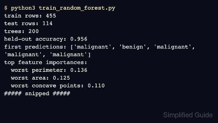
The built-in breast cancer dataset provides numeric features and two class labels for a compact training run. A stratified split reserves 20 percent of the rows for testing, and fixed random states make the split and forest repeatable while the program is being checked.
Held-out predictions provide the evidence that matters after fitting. Reporting the fitted tree count with test-set accuracy, precision, recall, and F1 score for both classes prevents one aggregate score from hiding a weak class result.
Steps to train a scikit-learn random forest classifier:
- Create train_random_forest.py with the imports and stratified dataset split.
- train_random_forest.py
from sklearn.datasets import load_breast_cancer
from sklearn.ensemble import RandomForestClassifier
from sklearn.metrics import classification_report
from sklearn.model_selection import train_test_split


data = load_breast_cancer()
X_train, X_test, y_train, y_test = train_test_split(
    data.data,
    data.target,
    test_size=0.2,
    stratify=data.target,
    random_state=42,
)
stratify=data.target keeps both diagnosis classes represented in the training and test subsets. The integer random_state selects the same rows again when the inputs are unchanged.
- Append the random forest definition after the split.
forest = RandomForestClassifier(
    n_estimators=200,
    max_depth=5,
    random_state=42,
    n_jobs=-1,
)
n_estimators=200 sets the forest size, while max_depth=5 limits how deep each tree can grow. n_jobs=-1 lets fitting use all available CPU cores.
- Append the fitting call after the forest definition.
forest.fit(X_train, y_train)
- Append the held-out prediction call after fitting.
predictions = forest.predict(X_test)
- Append the model and classification reporting after the prediction call.
print(f"training rows: {X_train.shape[0]}")
print(f"test rows: {X_test.shape[0]}")
print(f"fitted trees: {len(forest.estimators_)}")
print(f"held-out accuracy: {forest.score(X_test, y_test):.3f}")
print("classification report:")
print(
    classification_report(
        y_test,
        predictions,
        target_names=data.target_names,
    )
)
- Run the completed random forest training script.
$ python3 train_random_forest.py
training rows: 455
test rows: 114
fitted trees: 200
held-out accuracy: 0.956
classification report:
              precision    recall  f1-score   support

   malignant       0.95      0.93      0.94        42
      benign       0.96      0.97      0.97        72

    accuracy                           0.96       114
   macro avg       0.96      0.95      0.95       114
weighted avg       0.96      0.96      0.96       114
fitted trees: 200 confirms that training created the requested forest size. The classification report comes from predictions for 114 held-out rows and exposes recall for both malignant and benign cases.