How to calibrate a scikit-learn classifier

Probability estimates often feed decisions whose costs differ, such as escalating a high-risk case or leaving a low-risk case untouched. A classifier can rank those cases well while still assigning probabilities that are systematically too high or too low.

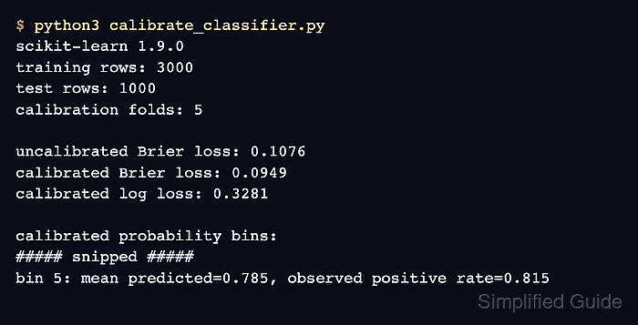
Scikit-learn's CalibratedClassifierCV fits classifier-and-calibrator pairs on separate folds, then averages their probability predictions. The sigmoid method used here adds a smooth correction that is suitable for a moderate calibration sample, while isotonic can overfit when calibration data is limited.

The final assessment belongs on rows excluded from both classifier and calibrator fitting. Brier loss and log loss summarize probability quality but also reflect discrimination and dataset uncertainty, so predicted-versus-observed rates from calibration_curve() provide the direct reliability check.

1. Create calibrate_classifier.py with the imports, synthetic classification data, and held-out split.

   calibrate_classifier.py

   import sklearn
   from sklearn.calibration import CalibratedClassifierCV, calibration_curve
   from sklearn.datasets import make_classification
   from sklearn.ensemble import RandomForestClassifier
   from sklearn.metrics import brier_score_loss, log_loss
   from sklearn.model_selection import train_test_split
    
    
   X, y = make_classification(
       n_samples=4_000,
       n_features=20,
       n_informative=7,
       n_redundant=5,
       weights=[0.78, 0.22],
       class_sep=0.65,
       flip_y=0.08,
       random_state=42,
   )
    
   X_train, X_test, y_train, y_test = train_test_split(
       X,
       y,
       test_size=0.25,
       stratify=y,
       random_state=42,
   )

2. Append the uncalibrated and sigmoid-calibrated classifiers after the held-out split.

   base_classifier = RandomForestClassifier(
       n_estimators=200,
       min_samples_leaf=8,
       random_state=42,
   )
   base_classifier.fit(X_train, y_train)
   base_probability = base_classifier.predict_proba(X_test)[:, 1]
    
   calibrated_classifier = CalibratedClassifierCV(
       estimator=RandomForestClassifier(
           n_estimators=200,
           min_samples_leaf=8,
           random_state=42,
       ),
       method="sigmoid",
       cv=5,
   )
   calibrated_classifier.fit(X_train, y_train)
   calibrated_probability = calibrated_classifier.predict_proba(X_test)[:, 1]

   Explicit cv=5 creates five stratified classifier-and-calibrator pairs for this binary target. Every calibrator learns from predictions made on its fold's held-out rows.

3. Append the held-out probability losses after the fitted probability arrays.

   print(f"scikit-learn {sklearn.__version__}")
   print(f"training rows: {X_train.shape[0]}")
   print(f"test rows: {X_test.shape[0]}")
   print(f"calibration folds: {len(calibrated_classifier.calibrated_classifiers_)}")
   print()
    
   for name, probability in (
       ("uncalibrated", base_probability),
       ("calibrated", calibrated_probability),
   ):
       print(f"{name} Brier loss: {brier_score_loss(y_test, probability):.4f}")
       print(f"{name} log loss: {log_loss(y_test, probability):.4f}")

   Brier and log losses are better when lower for the same held-out labels, but neither score isolates calibration from the classifier's ability to separate the classes.

4. Append the quantile reliability-bin report after the loss loop.

   fraction_positive, mean_predicted = calibration_curve(
       y_test,
       calibrated_probability,
       n_bins=5,
       strategy="quantile",
   )
    
   print()
   print("calibrated probability bins:")
   for bin_number, (predicted, observed) in enumerate(
       zip(mean_predicted, fraction_positive),
       start=1,
   ):
       print(
           f"bin {bin_number}: "
           f"mean predicted={predicted:.3f}, "
           f"observed positive rate={observed:.3f}"
       )

   Quantile bins contain approximately equal row counts. Smaller gaps between the mean prediction and observed positive rate indicate closer probability alignment within a bin.

5. Run the completed calibration script.

   $ python calibrate_classifier.py
   scikit-learn 1.9.0
   training rows: 3000
   test rows: 1000
   calibration folds: 5
   
   uncalibrated Brier loss: 0.1076
   uncalibrated log loss: 0.3655
   calibrated Brier loss: 0.0949
   calibrated log loss: 0.3281
   
   calibrated probability bins:
   bin 1: mean predicted=0.040, observed positive rate=0.050
   bin 2: mean predicted=0.072, observed positive rate=0.065
   bin 3: mean predicted=0.124, observed positive rate=0.090
   bin 4: mean predicted=0.250, observed positive rate=0.210
   bin 5: mean predicted=0.785, observed positive rate=0.815

   The calibrated model lowers both held-out losses in this run, and every reliability bin keeps the observed positive rate within 0.040 of its mean predicted probability.